Star Schema Design

                        Star Schema Design

Single fact table surrounded by denormalized dimension tables

The fact table primary key is the composite of the  foreign keys (primary keys of dimension tables)

Fact table contains transaction type information.

Many star schemas in a data mart

Easily understood by end users, more disk storage required

Galaxy Schema

Snow Flake Schema

Snowflake Schemas

The snowflake schema is a more complex data warehouse model than a star schema, and is a type of star schema. It is called a snowflake schema because the diagram of the schema resembles a snowflake.

Snowflake schemas normalize dimensions to eliminate redundancy. That is, the dimension data has been grouped into multiple tables instead of one large table. For example, a product dimension table in a star schema might be normalized into a products table, a product_category table, and a product_manufacturer table in a snowflake schema. While this saves space, it increases the number of dimension tables and requires more foreign key joins. The result is more complex queries and reduced query performance.  presents a graphical representation of a snowflake schema.

 Snowflake Schema

Star Schema

Star Schemas

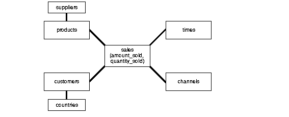
The star schema is perhaps the simplest data warehouse schema. It is called a star schema because the entity-relationship diagram of this schema resembles a star, with points radiating from a central table. The center of the star consists of a large fact table and the points of the star are the dimension tables.

A star schema is characterized by one or more very large fact tables that contain the primary information in the data warehouse, and a number of much smaller dimension tables (or lookup tables), each of which contains information about the entries for a particular attribute in the fact table.

A star query is a join between a fact table and a number of dimension tables. Each dimension table is joined to the fact table using a primary key to foreign key join, but the dimension tables are not joined to each other. The cost-based optimizer recognizes star queries and generates efficient execution plans for them.

A typical fact table contains keys and measures. For example, in the sh sample schema, the fact table, sales, contain the measures quantity_sold, amount, and cost, and the keys cust_id, time_id, prod_id,channel_id, and promo_id. The dimension tables are customers, times, products, channels, and promotions. The product dimension table, for example, contains information about each product number that appears in the fact table.

A star join is a primary key to foreign key join of the dimension tables to a fact table.

The main advantages of star schemas are that they:

• Provide a direct and intuitive mapping between the business entities being analyzed by end users and the schema design.
• Provide highly optimized performance for typical star queries.
• Are widely supported by a large number of business intelligence tools, which may anticipate or even require that the data-warehouse schema contain dimension tables

Star schemas are used for both simple data marts and very large data warehouses.

presents a graphical representation of a star schema.

Schema

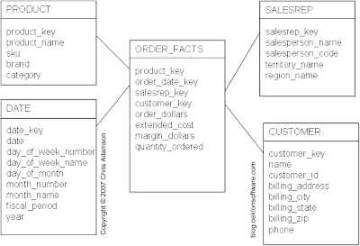
Figure 1: A demo schema usually represents orders or sales.
(Click to Enlarge)

You may have learned about the Star Schema by working with a sample like this one. If so, you probably have an intuitive grasp of star schema design principles. Here are ten terms and principles you should know that describe important features of the sample star.

1. Facts are measurements that describe a business process. They are almost always numeric—but not all numeric attributes are facts. You can find facts (or measurements) in almost any analytic request—"Show me sales dollars by product" (sales dollars). "How many widgets were sold my John Smith in May?" (quantity ordered).
   
2. Dimensions give facts context. They may be textual or numeric. They are used to specify how facts are "filtered" and "broken out" on reports. You can usually find dimensions after the words "by" or "for" in an analytic request. "Show me sales dollars by product" (product). "What are margin dollars by Month and Salesperson?" (month, sales rep).
   
3. Dimension tables are wide. Dimension tables usually group together a set of related dimension attributes, though there are situations where a dimension may include a set of attributes not related to one another. Dimension tables are not normalized, and usually have a lot of attributes—far more than appear in most sample schemas. This allows a rich set of detail to be used in analyzing facts. 100 or more columns is not uncommon for some dimensions. For this reason, we often call dimension tables wide.
   
4. Dimensions have Surrogate Keys. The primary key for each dimension table is an attribute specifically created for the dimensional schema. It is an integer assigned by the ETL process, and has no inherent meaning. It is not a reused key from a source system, such as a customer ID or product code. We call these attributes natural keys, and they may exist in the star, but do not serve as unique identifiers.
   
   In the sample schema, customer_key is a surrogate key generated for the star schema; customer_id is a natural key carried over from a source system.
   
   By assigning surrogate keys, we enable the star to handle changes to source data differently than the source system does. For example, in a source system a customer record may be overwritten, while we want the star schema to track changes. Performance considerations also come into play—a surrogate key avoids the need for multi-column joins.
   
5. Type 2 Changes track history. The term "Slowly Changing Dimension" (or SCD) describes how the data warehouse responds to changes in the source of dimensional data. There are several techniques that can be applied when the source of dimension detail changes. The most common is referred to as a "Type 2" change: an entirely new record is written to the dimension table.
   
   For example, if a customer moves, the record may simply be updated in a source system. But in the star schema, we choose to add a new row to the customer dimension, complete with a new surrogate key. All prior facts remain associated with the "old" customer record; all future facts will be associated with the new record.
   
6. Type 1 Changes overwrite history. The Type 1 change is used when source data changes are not deemed significant, or may be the correction of an error. In such cases, we perform an update to an existing row in a dimension. For example, if a customer's gender is updated in the source, we may choose to update it in the corresponding dimension records. All prior facts are now associated with the changed value.
   
   In addition to Type 1 and Type 2 changes, there are other SCD techniques. Hybrid approaches exist as well. Every design should identify which technique(s) will be used for each attribute of each dimension table.
   
7. Fact tables are narrow. A fact table row is usually entirely composed of numeric attributes: the facts, and foreign key references to the dimensions. Because of these characteristics, each fact table row is narrow, at least in contrast with wide dimension rows full of textual values. The narrowness of fact tables is important, because they will accumulate far more rows than dimension tables, and at a much faster rate.
   
8. Fact tables are usually sparse. Rows are recorded in the fact table only when there is something to measure. For example, not every customer orders every product from every salesperson each day. Rows are only recorded when there is an order. This helps manage the growth of the fact table. It also saves us from having to filter out a huge number of rows that have no sales dollars when displaying results in a report. (Usually, you don't want a customer sales report to list every product—only the ones they bought. You can use an outer join when you want the latter.)
   
9. Fact Table Grain The level of detail represented by a row in a fact table is referred to as its grain. Facts that are recorded with different levels of detail belong in separate fact tables. This avoids an array of reporting difficulties, as well as kludges such as including special rows in dimension tables for "not applicable." Determining the grain of a fact table is an important design step and helps avoid future confusion. (There are times when "not applicable" attributes are necessary, but they are most often a sign of the need for another fact table.)
   
   In the example, the grain is sales by customer, product, salesperson and date. A better design might capture sales at the order line level of detail.
   
10. Additivity. Facts are usually additive. This means they can be summed across any dimension value. For example,order_dollars can be aggregated across customers, products, salespeople, or time periods, producing meaningful results. Additive facts are stored in the fact table. We also store additive facts that might be computed from other facts. (order_dollars might be the sum of extended_cost andmargin_dollars, but why include only two out of the three.?
    
    Some facts are non-additive. For example, margin rate is a percentage. Two sales at 50% margin do not equate to a single sale at 100% margin—this fact is not additive. In the star, we store the fully additive components of margin (order_dollars and margin_dollars) and let front end tools compute the ratio. 

Degenrated Dimension

A degenerate dimension (DD) acts as a dimension key in the fact table, however does not join to acorresponding dimension table because all its interesting attributes have already been placed in other analytic dimensions. Sometimes people want to refer to degenerate dimensions as textual facts, however they're not facts since the fact table's primary key often consists of the DD combined with one or more additional dimension foreign keys.Degenerate dimensions commonly occur when the fact table's grain is a single transaction (or transaction line). Transaction control header numbers assigned by the operational business process are typically degenerate dimensions, such as order, ticket, credit card transaction, or check numbers. These degenerate dimensions are natural keys of the "parents" of the line items. Even though there is no corresponding dimension table of attributes, degenerate dimensions can be quite useful for grouping together related fact tables rows

Junk Dimension

The A junk dimension combines several low-cardinality flags and attributes into a single dimension table rather than modeling them as separate dimensions.

Slowly Changing Dimension

The term "slowly changing dimension" originated with Ralph Kimball, who identified three techniques for dealing with changed data. Commonly abbreviated as SCD's, these techniques are applied in any form of dimensional design, regardless of the data warehouse architecture.

In practice, there is a subtle but importance between the way we think about these changes and the way we describe them in a dimensional design. This sometimes leads to confusion.

Before I explain this important distinction, let me review the difference between surrogate and natural keys, and describe the two most common SCD techniques. (Future posts will look at other slow change techniques.)

Natural Keys and Surrogate Keys

We usually think of dimension tables in a star schema as corresponding to something in a source system. For example, each row in a customer dimension table relates to a single customer in a source system. Each column is loaded from one or more sources, based on a set of rules. The link back to a source system is preserved in the form of a natural key—usually a unique identifier in a source system, such as a customer_id.

But the star schema design does not rely on this natural key, orbusiness key, to uniquely identify rows in dimension tables. Instead, asurrogate key is introduced. This surrogate key gives the dimensional design flexibility to handle changes differently than they are handled in source systems, while preserving the ability to perform joins using a single column.

Type 1 and Type 2 Slow Changes

Slowly changing dimension techniques determine how the dimensional model will respond to changes in the source system. If the customer with id 8472 changes, what do we do with that change? Alert readers may already be concerned about what I mean by "change" here, but let's first recap the two most common techniques.

• Type 1: Update When the dimensional model responds to a change in source data by updating a column, Kimball calls this atype 1 change. For example, if a customer's date of birth changes, it is probably appropriate to update the corresponding row for that customer in the dimension table.
  
  Under this scenario, any facts that were already associated with the dimension table row have effectively been revised as well. A report of sales dollars by date of birth, for example, will provide different results immediately before and after the type 1 change is applied. The type 1 change does not preserve history of the attribute value.

• Type 2: New Row A more common response to a changed data element is to insert a new row into the dimension table. For example, when the address of customer 8472 changes, we create a new row for the customer in the dimension table. This row has a different surrogate key, and the new address. Customer 8472 now has two rows in the dimension, each with its own surrogate key.
  
  This preserves the history of the attribute, and does not revise any previously stored facts. New facts will be associated with the new version of customer 8472; old facts remain associated with the old version.
  

For the most part, these two techniques form the basis of a dimensional model's response to change. (Future posts will consider the less common type 3 change, and additional techniques.) While these concepts are fairly easy to understand, it is important to look a bit deeper.

We think about slow changes with respect to the source

Notice the way that the original problem was framed. I asked how the dimensional schema would "respond to changes in the source data." This is how we usually think about the problem, and for good reason. After all, the source data exists before it is loaded into the dimensional schema. If birth_date changes, we overwrite; ifaddress changes, we insert a new record.

Now observe that a change to the source does not always result in a change in the dimensional schema. In the example, a change in address resulted in a new row—not a changed row. No data is changed.

Still, we refer to this process as the occurrence of a type 2 change. Why? Because we think about slow changes with respect to the sourcedata. And there, a change did occur.

We document slow changes with respect to the star

The most common way to document the dimensional schema's response to change is on the dimensional side, on an attribute by attribute basis. For each column in a dimension table, we note how changes in the source data will be handled. Our customer example might be documented as follows:

In the diagram, each non-key attribute is tagged with a 1 or a 2. This indicates whether changes in the source of the attribute should be handled as type 1 or type 2 changes.

Documenting SCD behavior in this way is handy. ETL developers use this information to design a scheme for performing incremental loads. Report developers use this information to understand how facts will be grouped when combined with different dimension attributes.

The only drawback to documenting SCD rules in this way is that it can lead to confusion. By tagging an attribute as a "type 2 SCD" we risk implying that attribute values may change. After all, the "C" in "SCD" stands for "change." 

But of course, this attribute does not change. Rather, its classification as a type 2 attribute means "for a given natural key, if the source for this attribute undergoes a change, it will be necessary to insert a new row. 

Surrogate Keys

Surrogate keys are for dimension tables 

A surrogate key is an attribute that is created to uniquely identify rows in a dimensiontable. It does not come from a source system; it is created expressly for the dimensional schema.

Surrogate keys for dimension tables serve two important purposes:

1. They make it easier to track history.  They allow the dimension to capture changes to something, even if the source does not.  Absent a surrogate key, this would be difficult; the primary key of the dimension would be concatenation of natural keys and type 2 attributes.
2. They make it easy to join to the dimension.  The dimensions' surrogate keys appear in fact tables as  foreign keys.  They allow the fact to be joined to the appropriate dimension values, without having to use a multi-part key.

FactLess Table

When a fact table does not contain any facts, it is called afactless fact table. There are two types of factless fact tables: those that describe events, and those that describe conditions. Both may play important roles in your dimensional models. 

Factless fact tables for events

Sometimes there seem to be no facts associated with an important business process. Events or activities occur that you wish to track, but you find no measurements. In situations like this, build a standard transaction-grained fact table that contains no facts.

For example, you may be tracking contact events with customers. How often and why we have contact with each customer may be an important factor in focusing retention efforts, targeting marketing campaigns, and so forth.

The factless fact table shown here captures a row each time contact with a customer occurs.  Dimensions represent the date and time of each contact, the customer contacted, and the type of communication (e.g. inbound phone call, outbound phone call, robo-call, email campaign, etc.).

While there are no facts, this kind of star schema is indeed measuring something: the occurrence of events. In this case, the event is a contact. Since the events correspond to the grain of the fact table, a fact is not required;